Magick 1.0: 🎩 ✨🐇 Advanced Graphics and Image Processing in R

Last week, version 1.0 of the magick package appeared on CRAN: an ambitious effort to modernize and simplify high quality image processing in R. This R package builds upon the Magick++ STL which exposes a powerful C++ API to the famous ImageMagick library.

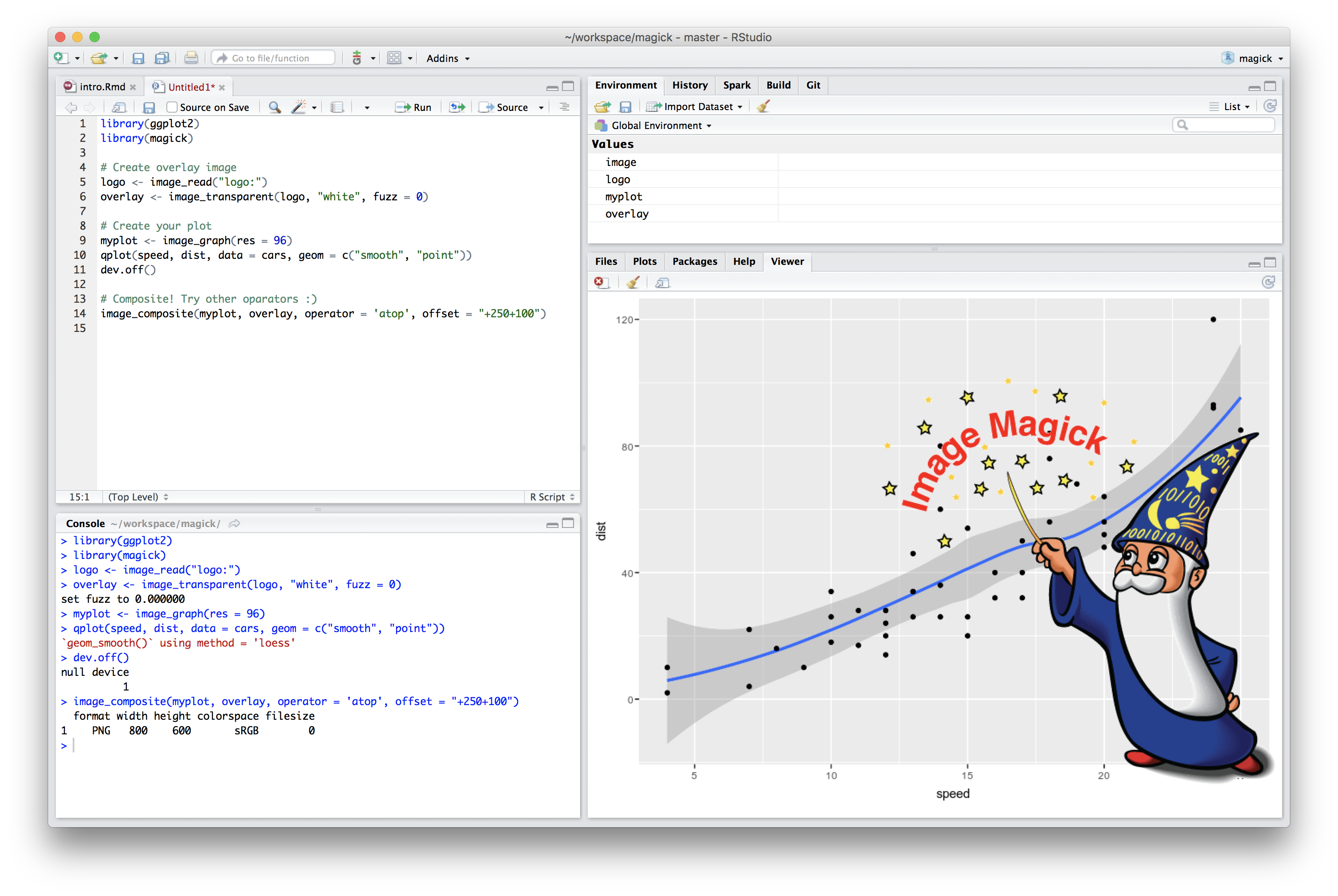
The best place to start learning about magick is the vignette which gives a brief overview of the overwhelming amount of functionality in this package.

Towards Release 1.0

Last year around this time rOpenSci announced the first release of the magick package: a new powerful toolkit for image reading, writing, converting, editing, transformation, annotation, and animation in R. Since the initial release there have been several updates with additional functionality, and many useRs have started to discover the power of this package to take visualization in R to the next level.

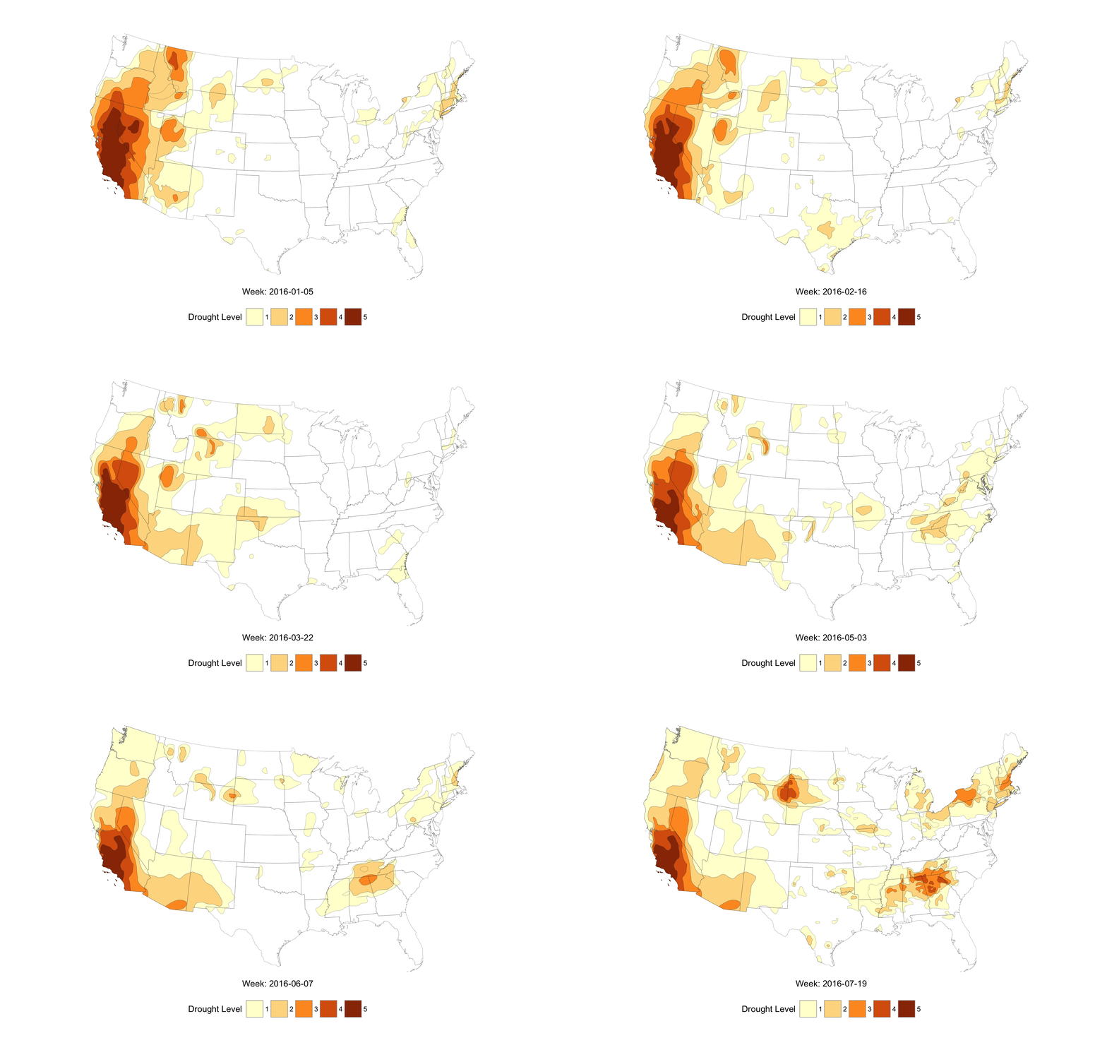
For example Bob Rudis uses magick to visualize California drought data from the U.S. Drought Monitor (click on the image to go find out more):

R-ladies Lucy D’Agostino McGowan and Maëlle Salmon demonstrate how to make a beautiful collage:

And Daniel P. Hadley lets Vincent Vega explains Cars:

Now, 1 year later, the 1.0 release marks an important milestone: the addition of a new native graphics device (which serves as a hybrid between a magick image object and an R plot) bridges the gap between graphics and image processing in R.

This blog post explains how the magick device allows you to seamlessly combine graphing with image processing in R. You can either use it to post-process your R graphics, or draw on imported images using the native R plotting machinery. We hope that this unified interface will make it easier to produce beautiful, reproducible images with R.

Native Magick Graphics

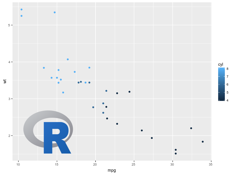
The image_graph() function opens a new graphics device similar to e.g. png() or x11(). It returns an image object to which the plot(s) will be written. Each page in the plotting device will become a frame (layer) in the image object.

# Produce image using graphics device
fig <- image_graph(res = 96)
ggplot2::qplot(mpg, wt, data = mtcars, colour = cyl)
dev.off()

The fig object now contains the image that we can easily post-process. For example we can overlay another image:

logo <- image_read("https://www.r-project.org/logo/Rlogo.png")
out <- image_composite(fig, image_scale(logo, "x150"), offset = "+80+380")

# Show preview
image_browse(out)

# Write to file
image_write(out, "myplot.png")

Drawing Device

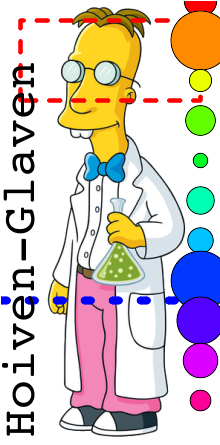
The image_draw() function opens a graphics device to draw on top of an existing image using pixel coordinates.

# Open a file
library(magick)
frink <- image_read("https://jeroen.github.io/images/frink.png")
drawing <- image_draw(frink)

We can now use R’s native low-level graphics functions for drawing on top of the image:

rect(20, 20, 200, 100, border = "red", lty = "dashed", lwd = 5)
abline(h = 300, col = 'blue', lwd = '10', lty = "dotted")
text(10, 250, "Hoiven-Glaven", family = "courier", cex = 4, srt = 90)
palette(rainbow(11, end = 0.9))
symbols(rep(200, 11), seq(0, 400, 40), circles = runif(11, 5, 35),
  bg = 1:11, inches = FALSE, add = TRUE)

At any point you can inspect the current result:

image_browse(drawing)

Once you are done you can close the device and save the result.

dev.off()
image_write(drawing, 'drawing.png')

By default image_draw() sets all margins to 0 and uses graphics coordinates to match image size in pixels (width x height) where (0,0) is the top left corner. Note that this means the y axis increases from top to bottom which is the opposite of typical graphics coordinates. You can override all this by passing custom xlim, ylim or mar values to image_draw().

Animated Graphics

The graphics device supports multiple frames which makes it easy to create animated graphics. The example below shows how you would implement the example from the very cool gganimate package using the magick.

library(gapminder)
library(ggplot2)
library(magick)
img <- image_graph(res = 96)
datalist <- split(gapminder, gapminder$year)
out <- lapply(datalist, function(data){
  p <- ggplot(data, aes(gdpPercap, lifeExp, size = pop, color = continent)) +
    scale_size("population", limits = range(gapminder$pop)) +
    scale_x_log10(limits = range(gapminder$gdpPercap)) +
    geom_point() + ylim(20, 90) +  ggtitle(data$year) + theme_classic()
  print(p)
})
dev.off()
animation <- image_animate(img, fps = 2)
image_write(animation, "animation.gif")

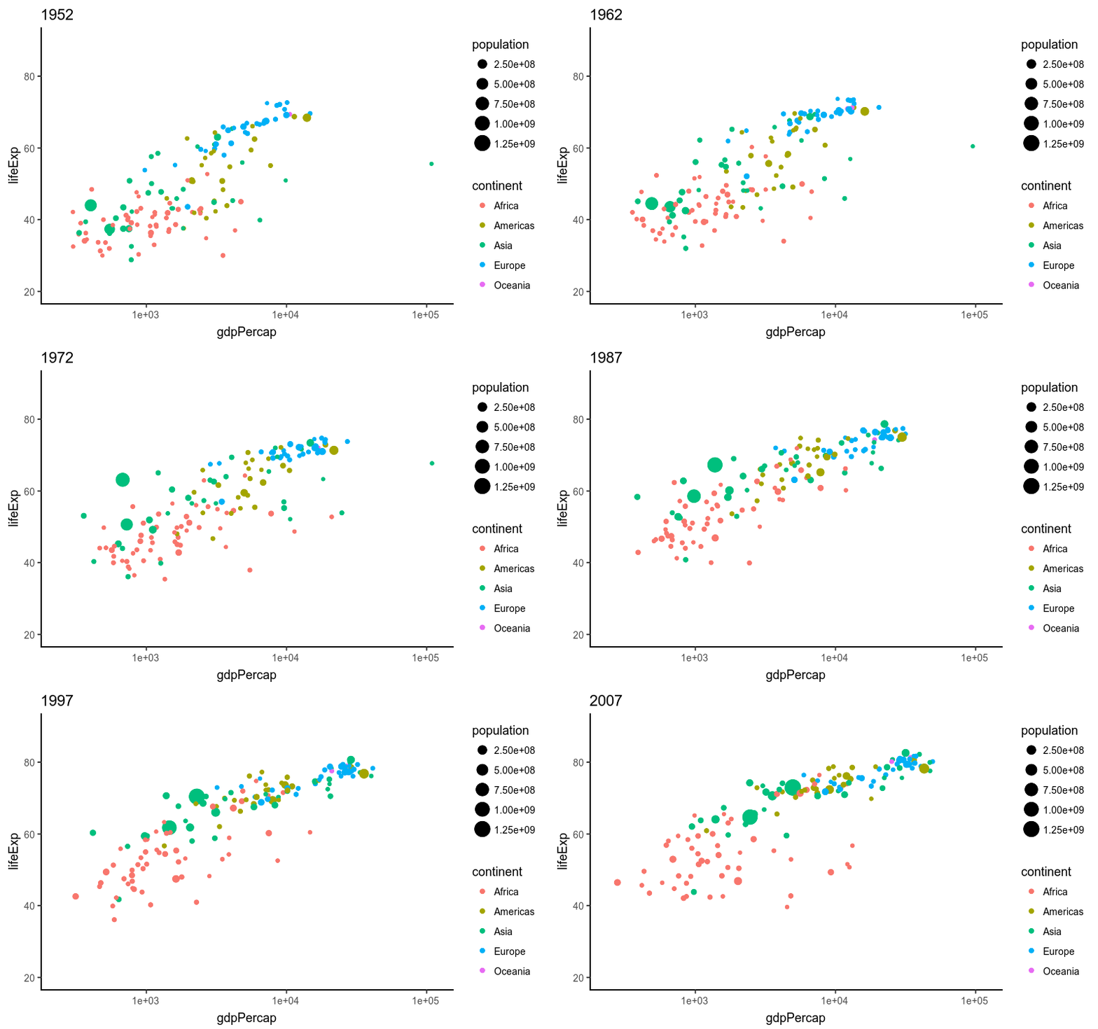
We hope that the magick package can provide a more robust back-end for packages like gganimate to produce interactive graphics in R without requiring the user to manually install external image editing software.

Porting ImageMagick Commands to R

The magick 1.0 release now has the core image processing functionality that you expect from an image processing package. But there is still a lot of room for improvement to make magick the image processing package in R.

A lot of R users and packages currently shell out to ImageMagick command line tools for performing image manipulations. The goal is to support all these operations in the magick package, so that the images can be produced (and reproduced!) on any platform without requiring the user to install additional software.

Note that ImageMagick library is over 26 years old and has accumulated an enormous number of features in those years. Porting all of this to R is quite a bit of work, for which feedback from users is important. If there is an imagemagick operation that you like to do in R but you can’t figure out how, please open an issue on GitHub. If the functionality is currently not supported yet, we will try to add it to the next version.

Image Analysis

Currently magick is focused on generating and editing images. There is yet another entirely different set of features which we like to support related to analyzing images. Image analysis can involve anything from calculating color distributions to more sophisticated feature extraction and vision tools. I am not very familiar with this field, so again we could use suggestions from users and experts.

One feature that is already available is the image_ocr() function which extracts text from the image using the rOpenSci tesseract package. Another cool example of using image analysis is the collage package which calculates color histograms to select appropriate tile images for creating a collage.

As part of supporting supporting analysis tools we plan to extract the bitmap (raster) classes into a separate package. This will enable package authors to write R extensions to analyze and manipulate on the raw image data, without necessarily depending on magick. Yet the user can always rely on magick as a powerful toolkit to import/export images and graphics into such low level bitmaps.

The greatest achievement of my PhD so far: discovering the 'magick' R package and adding gifs to my plots (thanks @danielphadley!) #rstats pic.twitter.com/gCEfKyWa9x

— George Bailey (@grbails) July 13, 2017