Where to go observe birds in Radolfzell? An answer with R and open data

This post is the 1st post of a series showcasing various rOpenSci packages as if Maëlle were a birder trying to make the most of R in general and rOpenSci in particular. Although the series use cases will mostly feature birds, it’ll be the occasion to highlight rOpenSci’s packages that are more widely applicable, so read on no matter what your field is! Moreoever, each post should stand on its own.

A logical first step in this birder’s guide to rOpenSci is to use R to find where to observe birds! In this blog post, we shall use rOpenSci packages accessing open geographical data to locate and visualize where to observe birds near a given location.

First of all, where are we now?

The Max Planck Institute for Ornithology (henceforth shortened to MPI), where Maëlle will give a talk is located at Am Obstberg 1 78315 Radolfzell. Let’s geolocate it using rOpenSci’s opencage package that interfaces the OpenCage Geocoder, a commercial service based on open data. When choosing to get only one result via limit = 1, one gets what the API considers to be the best one.

mpi <- opencage::opencage_forward("Am Obstberg 1 78315 Radolfzell", limit = 1)$results
class(mpi)

## [1] "tbl_df"     "tbl"        "data.frame"

head(names(mpi))

## [1] "annotations.DMS.lat"    "annotations.DMS.lng"   
## [3] "annotations.MGRS"       "annotations.Maidenhead"
## [5] "annotations.Mercator.x" "annotations.Mercator.y"

This gets us Am Obstberg 1, 78315 Radolfzell, Germany (mpi$formatted) which is in 🇩🇪 (mpi$annotations.flag gets us a flag!).

Birding in a bird hide?

Where to find a bird hide?

You can most certainly go birding anywhere, but if you can find a bird hide (or bird blind depending on the English you speak), it might be a very appropriate observation point. Now that we know where the MPI is, we can look for bird hide(s) in the vicinity. For that, we shall use rOpenSci’s osmdata package by Mark Padgham and collaborators! Note that incidentally, Mark did his PhD in ecology. This package is an interface to OpenStreetMap’s Overpass API. OpenStreetMap is a collective map of the world. It contains information about towns’ limits, roads, placenames… but also tags of everything, from bars as seen in this blog post to trees. You can browse existing features via OpenStreetMap’s wiki. Some parts of the world are better mapped than others depending on the local OpenStreetMap community. Actually, OpenCage’s blog features an interesting series of country profiles.

To look for a bird hide, we first create a bounding box of 10km around the MPI, using rOpenSci’s bbox package.

bbox <- bbox::lonlat2bbox(mpi$geometry.lng,
                          mpi$geometry.lat,
                          dist = 10, method = "lawn")

We then use the key and value associated with bird hides in OpenStreetMap: respectively leisure and bird_hide.

library("osmdata")

## Data (c) OpenStreetMap contributors, ODbL 1.0. http://www.openstreetmap.org/copyright

library("magrittr")
(results <- opq(bbox = bbox) %>%
  add_osm_feature(key = 'leisure', value = 'bird_hide') %>%
  osmdata_sf ())

## Object of class 'osmdata' with:
##                  $bbox : 47.6865,8.8753,47.8494,9.1177
##         $overpass_call : The call submitted to the overpass API
##             $timestamp : [ Thu 5 Jul 2018 08:06:35 ]
##            $osm_points : 'sf' Simple Features Collection with 1 points
##             $osm_lines : 'sf' Simple Features Collection with 0 linestrings
##          $osm_polygons : 'sf' Simple Features Collection with 0 polygons
##        $osm_multilines : 'sf' Simple Features Collection with 0 multilinestrings
##     $osm_multipolygons : 'sf' Simple Features Collection with 0 multipolygons

results$osm_points

##              leisure            geometry
## 5004940425 bird_hide 8.920901, 47.741569

Yay, we now know where to find a bird hide not too far from the MPI!

Visualizing our location and the bird hide

So one could enter the coordinates of that bird hide in one’s favourite mapping software or app but to show you where the bird hide is we can actually step back and use osmplotr, another package contributed to rOpenSci by Mark Padgham!

The way osmplotr works is letting you create a basemap, on which you’ll add different layers extracted from OpenStreetMap using osmplotr::extract_osm_objects or osmdata functions directly. Its strengths are therefore the use of open data, and the customization of what you’re using as background!

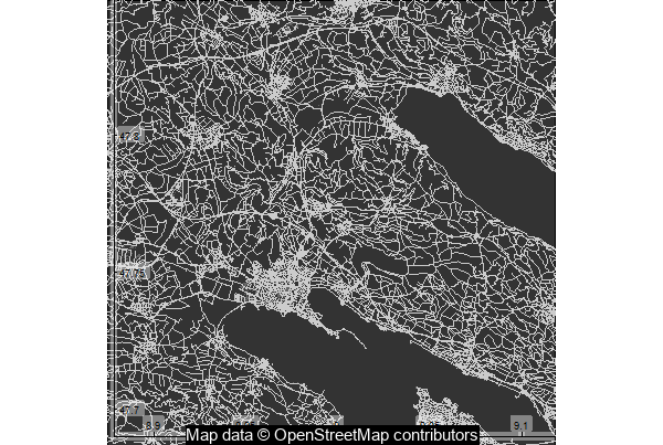
Let’s create a basemap for our bounding box, and then add roads and buildings to it.

library("osmplotr")

## Data (c) OpenStreetMap contributors, ODbL 1.0. http://www.openstreetmap.org/copyright

bbox <- get_bbox(bbox)
dat_B <- extract_osm_objects (key = 'building', bbox = bbox)
dat_H <- extract_osm_objects (key = 'highway', bbox = bbox)

map0 <- osm_basemap(bbox = bbox, bg = 'gray20') %>%
  add_osm_objects (dat_B, col = 'gray40') %>%
  add_osm_objects (dat_H, col = 'gray80')

map0 %>%
  add_axes() %>%
  print_osm_map (filename = 'map_a1.png', width = 600,
               units = 'px', dpi = 72)

library("magrittr")
magick::image_read('map_a1.png') %>%
  magick::image_annotate("Map data © OpenStreetMap contributors",
                         color = "white",
                         boxcolor =  "black",
                         size = 15,
                         gravity = "south")

Quite pretty! The lakes can be seen because of the absence of roads and buildings on them.

Now, let’s plot the bird hide and the MPI on them. Since we used osmdata::osmdata_sf, we had gotten the data in a receivable class, sf.

points_map <- add_osm_objects(map0, results$osm_points, 
                              col = 'salmon',
                              size = 5)

For plotting the MPI, we’ll convert opencage output to an sf point with the same coordinate reference system as the OpenStreetMap data extracted with osmdata.

coords <- data.frame(lon = mpi$geometry.lng,
                     lat = mpi$geometry.lat)
crs <- sf::st_crs(results$osm_points)

mpi_sf <- sf::st_as_sf(coords,
                       coords = c("lon", "lat"), 
                      crs = crs)

points_map <- add_osm_objects(points_map, mpi_sf, 
                             col = 'white',
                             size = 5)

We can now visualize both points on the map, the MPI in white and the bird hide in salmon, South-West from the MPI.

points_map %>%
  add_axes() %>%
  print_osm_map (filename = 'map_a2.png', 
                 width = 600,
                 units = 'px', dpi = 72) 

magick::image_read('map_a2.png') %>%
  magick::image_annotate("Map data © OpenStreetMap contributors",
                         color = "white",
                         boxcolor =  "black",
                         size = 15,
                         gravity = "south")

Aha, now we see where the bird hide is, fantastic! But as Mark noted, birds can actually be observed from other places.

Birding where birds should be?

Birds are most likely to be found where water lies close to natural areas, and we can translate this to R code! We shall get all water and (separately) all non-watery natural areas and find the shortest distances between them before plotting the results using add_osm_surface.

First, let’s get all water and (separately) all non-watery natural areas.

dat <- opq(bbox = bbox) %>%
     add_osm_feature(key = 'natural') %>%
     osmdata_sf (quiet = FALSE)

## Issuing query to Overpass API ...

## Rate limit: 2

## Query complete!

## converting OSM data to sf format

indx_W <- which (dat$osm_polygons$natural %in% c ("water", "wetland"))
indx_N <- which (!dat$osm_polygons$natural %in% c ("water", "wetland"))

xy_W <- sf::st_coordinates (dat$osm_polygons [indx_W, ])
xy_N <- sf::st_coordinates (dat$osm_polygons [indx_N, ])

Then we use Mark’s geodist package to get pairwise distances between all points, find minima, and make a data.frame to submit to add_osm_surface(). We have 7068 watery points and 10065 non-watery points so the speed of geodist is crucial here!

t1 <- Sys.time()
d <- geodist::geodist (xy_W, xy_N)
# so fast!!!
Sys.time() - t1

## Time difference of 13.57983 secs

d1 <- apply (d, 1, min)
d2 <- apply (d, 2, min)
xy <- cbind (rbind (xy_W, xy_N), c (d1, d2))
xy <- xy [, c (1, 2, 5)]
colnames (xy) <- c ("x", "y", "z")
xy <- xy [!duplicated (xy), ]

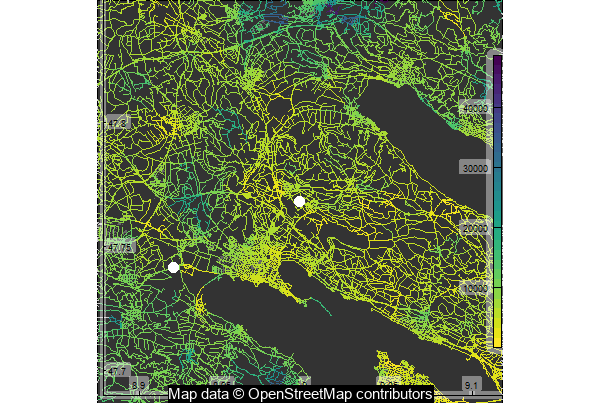
Finally we plot the results on the roads we had gotten earlier, although we do not recommend staying on the middle of a road to observe birds! We re-add the points corresponding to the MPI and bird hide after the surface coloring. With osmplotr, order matters because layers are added on top of each other. Note that plotting the distances takes a while.

# colorblind-friendly palette!
cols <- viridis::viridis_pal (direction = -1) (30)

add_osm_surface (map0, dat_H,
                 dat = xy, col = cols) %>%
    add_axes()  %>%
  add_colourbar(cols = cols,
                zlim = range(xy[,"z"])) %>%
  add_osm_objects(mpi_sf, 
                  col = 'white', size = 5) %>%
  add_osm_objects(results$osm_points, 
                  col = 'white', size = 5)%>%
  print_osm_map (filename = 'map_a3.png', width = 600,
                 units = 'px', dpi = 72)

magick::image_read('map_a3.png') %>%
  magick::image_annotate("Map data © OpenStreetMap contributors",
                         color = "white",
                         boxcolor =  "black",
                         size = 15,
                         gravity = "south")

On the map, the yellower/lighter a road is, the better it is to observe birds according to Mark’s assumption that birds are most likely to be found where water lies close to natural areas. With this metric, the MPI itself is not too badly located, which after all is not too surprising for an MPI of ornithology. Maybe one should just walk to the one of the nearest lakes to meet some birds.

Conclusion

Open geographical data in R

In this post we showcased three rOpenSci packages helping you use open geographical data in R: opencage, osmdata, osmplotr, therefore mostly making use of the awesome OpenStreetMap data (The OpenCage Geocoder uses a bit more, but it only warrants attributing OpenStreetMap). We therefore added the annotation “Map data © OpenStreetMap contributors” to all maps of this post using rOpenSci’s magick package. You might also have noticed in the code earlier that both osmdata and osmplotr have start-up messages indicating the data origin and licence.

Another package of rOpenSci’s interacting with open geographical data, that might be of interest for making maps, is rnaturalearth that facilitates interaction with Natural Earth map data.

Other R packages for spatial analyses

We also used two other rOpenSci packages: bbox to get a bounding box and magick for image manipulation. Explore more of our packages suite, including and beyond the geospatial category, here.

We also used the geodist package for ultra lightweight, ultra fast calculation of geo distances. This package is developed in the hypertidy GitHub organization which is a good place to find useful R geospatial packages. Other good resources for geospatial analyses with R include the r-spatial.org website and this great book by Robin Lovelace, Jakub Nowosad and Jannes Muenchow, and more links presented in this blog post of Steph Locke’s.

More birding soon!

Stay tuned for the next post in this series, about getting bird observation data in R! In the meantime, happy birding!